Overview of the diverse functions of prion proteins in Creutzfeldt-Jakob disease, Alzheimer’s disease, and other dementias. The prion protein serves as a co-receptor for neurotoxic oligomeric species such as beta-amyloid and α-synuclein and mediates neurotoxicity via Src kinase Fyn. The prion protein is also involved in the spreading of tau oligomers through LRP. Additionally, it is implicated in the neurotoxicity caused by pathological prions (PrPSc).
HSA KIT: Precise Analysis of Vacuoles and PrP Deposits with Deep Learning
Vacuole
During the progression of neurodegenerative diseases, neurons overloaded with misfolded prion proteins swell and die, creating characteristic holes in brain tissue that can be recognized in histological sections. These vacuoles vary in size depending on the subtype—ranging from small to large or confluent—and also differ between brain regions.
PrP (Prion Protein)
The specially developed PrP model enables precise visualization of misfolded proteins. Using targeted immunohistochemical staining, these appear as clearly visible brown spots on histological sections. These proteins vary in density, size, definition, and distribution depending on the brain region.
Region
The HSA KIT enables precise detection of affected regions and a detailed analysis of white matter and cortex within a single sample. Additionally, specific characteristics of different brain regions are considered, such as the structure in the thalamus and striatum or the different layers in the cerebellum.


Zoomed in: Automatic detection of the cerebellum in three different areas: Cerebellum Molecular Layer (brown), Cerebellum Granular Layer (purple), and Cerebellum White Matter (teal) using the HSA KIT.
Automatic Subdivision of the Cortex into 6 Layers with HSA KIT
The HSA KIT software enables precise and automatic subdivision of the cortex into six layers to conduct a detailed analysis of the various cellular and structural characteristics in the brain. This method captures and compares specific features, such as the distribution and density of structures (e.g., vacuoles or PrP deposits) within each layer.


Zoomed in: Automatic detection of the cortical lobe cortex (yellow) and cortical lobe white matter, followed by the subdivision of the cortex into 6 layers. Finally, automatic detection of vacuoles was performed using the HSA KIT.
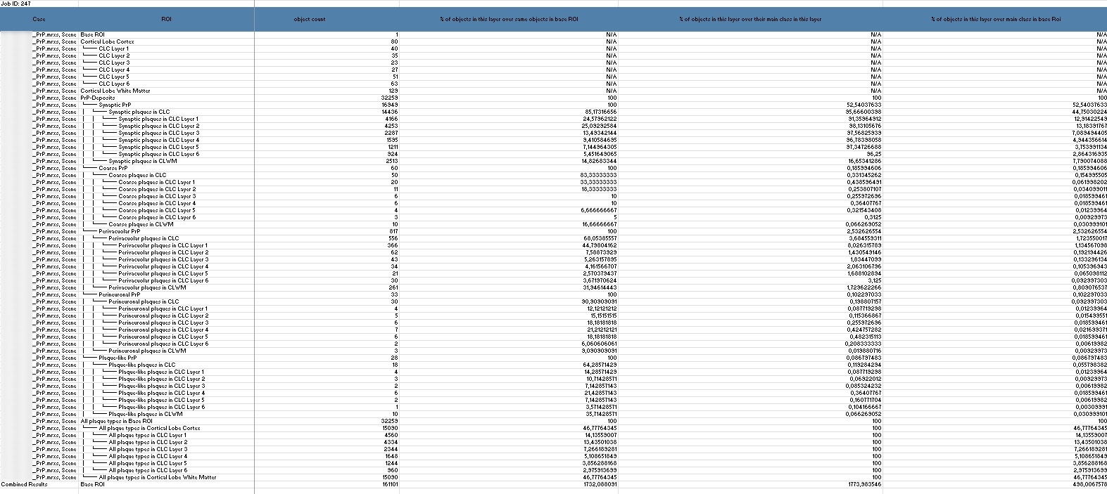
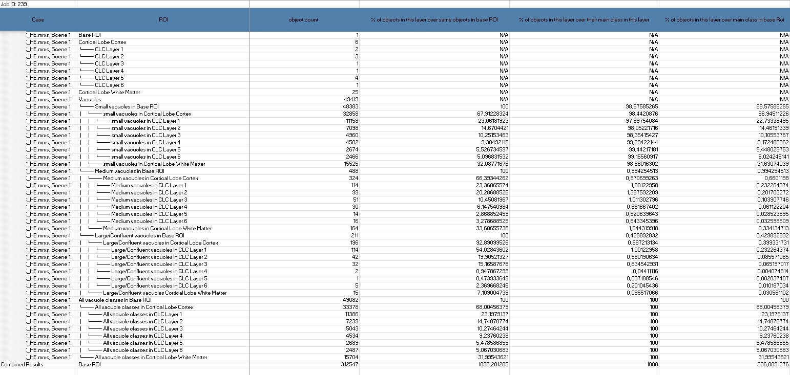
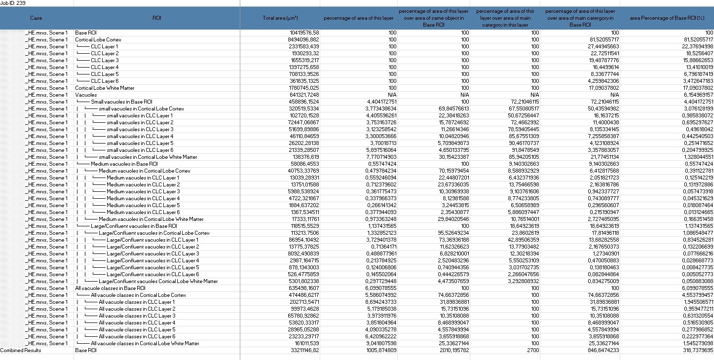
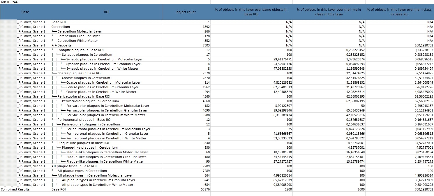
Result Table
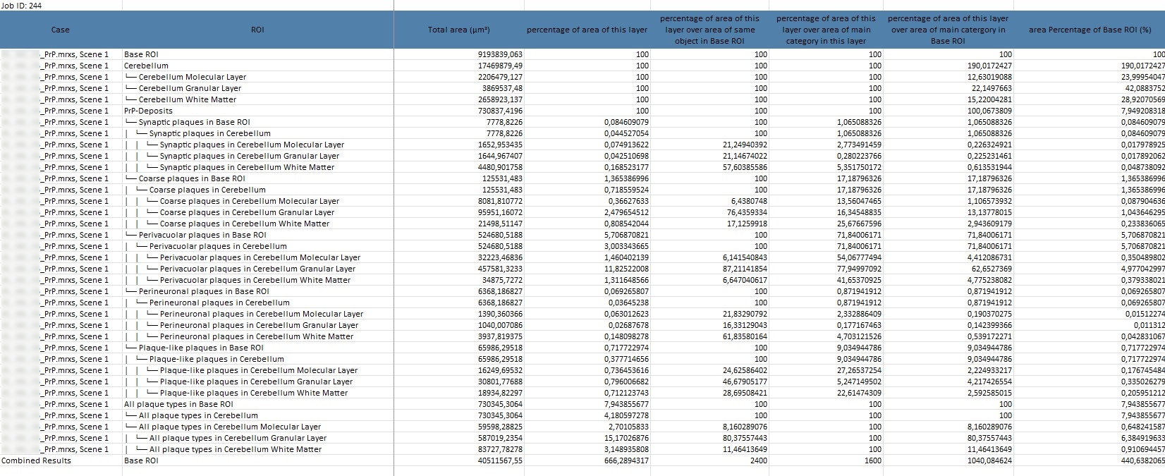
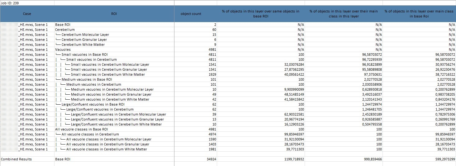
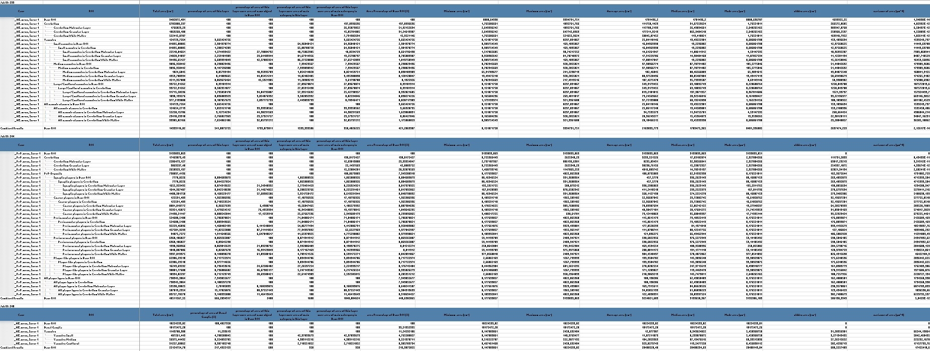
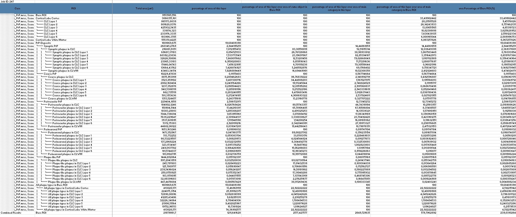
The differentiation of Creutzfeldt-Jakob subtypes requires a thorough analysis of selected metrics, providing valuable insights into the distribution and characteristics of brain structures. These metrics are crucial for precisely examining structures such as vacuoles and PrP deposits and drawing significant conclusions regarding specific subtypes.
Detailed Information on the Table:
Case: The sample or scene examined.
ROI (Region of Interest): The specific region or layer, e.g., the “Cerebellum Molecular Layer.”
Total Area (µm²) and Percentage of Area of This Layer: These values provide information about the area occupied by structures within a layer.
Object Count: Indicates how many objects are present in a particular layer, giving insight into the density of structures.
% of Area of This Layer Over Area of Same Object in Base ROI and % of Objects in This Layer Over Same Objects in Base ROI: These values are essential for comparing the distribution of objects in a layer to the entire examined region.
% of Objects in This Layer Over Their Main Class in This Layer and % of Objects in This Layer Over Their Main Class in Base ROI: These metrics show the relative distribution and concentration of objects within a layer compared to the main class and the entire region.
Shape Factor: Measures the shape and roundness of objects, which is important for analyzing structures.
This data helps to analyze the distribution and density of structures in the cortex and is crucial for identifying differences between layers, an essential step for investigating disease patterns.
Conclusions on CJD Subtypes with HSA KIT Software:
The main goal of this analysis, conducted with HSA KIT software, is to draw conclusions on specific subtypes of CJD using the metrics mentioned. Since different subtypes show significant differences in the number and distribution of structures in certain layers, analyzing these differences allows for subtype classification through AI.
By comparing the various regions and layers and statistically evaluating the shapes and distributions processed with the HSA KIT, more precise diagnosis and classification of subtypes are made possible.
Additional calculations are applied. For more detailed information, refer to:
Area results
Total Area
The sum of all polygon areas.
$$\text{Total Area} = \sum_{i=1}^{n} \text{Area}_i$$
Percentage Area of Base ROI
The percentage of the total area of polygons relative to the base ROI.
$$\text{Percentage Area} = \left( \frac{\text{Total Area}}{\text{Base ROI Area}} \right) \times 100 \%$$
Minimum Area
The smallest polygon area.
$$\text{Minimum Area} = \min(\text{Area}_1, \text{Area}_2, \ldots, \text{Area}_n)$$
Maximum Area
The largest polygon area.
$$\text{Maximum Area} = \max(\text{Area}_1, \text{Area}_2, \ldots, \text{Area}_n)$$
Average Area
The mean area of all polygons.
$$\text{Average Area} = \frac{\sum_{i=1}^{n} \text{Area}_i}{n}$$
Median Area
The median area of all polygons.
$$\text{Median} =
\begin{cases}
\text{Area}_{\left(\frac{n+1}{2}\right)} & \text{if } n \text{ is odd} \\
\frac{\text{Area}_{\left(\frac{n}{2}\right)} + \text{Area}_{\left(\frac{n}{2} + 1\right)}}{2} & \text{if } n \text{ is even}
\end{cases}$$
Mode Area
The most frequently occurring area value.
$$\text{Mode Area} = \text{The value that appears most frequently in the dataset}$$
Standard Deviation (StdDev) Area
The measure of dispersion of polygon areas.
$$\text{StdDev} = \sqrt{\frac{1}{n} \sum_{i=1}^{n} (\text{Area}_i – \text{Average Area})^2}$$
Variance of Area
The square of the standard deviation.
$$\text{Variance} = \frac{1}{n} \sum_{i=1}^{n} (\text{Area}_i – \text{Average Area})^2$$
Mean Absolute Deviation of Area
The average of the absolute deviations from the mean.
$$\text{MAD} = \frac{1}{n} \sum_{i=1}^{n} |\text{Area}_i – \text{Average Area}|$$
Skewness
The measure of the asymmetry of the distribution of area values.
$$\text{Skewness} = \frac{\sum_{i=1}^{n} (\text{Area}_i – \text{Average Area})^3}{n \cdot \text{StdDev}^3}$$
Kurtosis
The measure of the “tailedness” of the distribution of area values.
$$\text{Kurtosis} = \frac{\sum_{i=1}^{n} (\text{Area}_i – \text{Average Area})^4}{n \cdot \text{StdDev}^4}$$
Object Size Quartiles (1st, 2nd, 3rd)
The quartile values of polygon areas.
$$\text{Q1} = \text{Area}_{\left(\frac{n+1}{4}\right)}$$
$$\text{Q3} = \text{Area}_{\left(\frac{2(n+1)}{4}\right)}$$
$$\text{Q3} = \text{Area}_{\left(\frac{3(n+1)}{4}\right)}$$
Interquartile Range (1st – 3rd)
The range between the first and third quartile.
$$\text{IQR} = \text{Q3} – \text{Q1}$$
Decile Sizes (1st to 9th)
Values that divide the dataset into ten equal parts.
$$\text{D1} = \text{Area}_{\left(\frac{n+1}{10}\right)}$$
$$\text{D2} = \text{Area}_{\left(\frac{2(n+1)}{10}\right)}$$
$$\text{D3} = \text{Area}_{\left(\frac{3(n+1)}{10}\right)}$$
$$\text{D4} = \text{Area}_{\left(\frac{4(n+1)}{10}\right)}$$
$$\text{D5} = \text{Area}_{\left(\frac{5(n+1)}{10}\right)}$$
$$\text{D6} = \text{Area}_{\left(\frac{6(n+1)}{10}\right)}$$
$$\text{D7} = \text{Area}_{\left(\frac{7(n+1)}{10}\right)}$$
$$\text{D8} = \text{Area}_{\left(\frac{8(n+1)}{10}\right)}$$
$$\text{D9} = \text{Area}_{\left(\frac{9(n+1)}{10}\right)}$$
Confidence Intervals of Area
The range within which the true mean of the population lies with a certain confidence level.
$$\text{CI} = \text{Average Area} \pm (z \times \frac{\text{StdDev}}{\sqrt{n}})$$
Shape Factor
A measure of the compactness of the shape.
$$\text{Shape Factor} = \frac{4\pi \times \text{Area}}{\text{Perimeter}^2}$$
Area to Perimeter Ratio
The ratio of area to perimeter.
$$\text{Ratio} = \frac{\text{Area}}{\text{Perimeter}}$$
Eccentricity
The ratio of the distance between the foci of the ellipse and its major axis length.
$$\text{Eccentricity} = \sqrt{1 – \frac{b^2}{a^2}}$$
Other results
Object count
The number of polygons
Object density
The number of polygons per unit area.
$$\text{Object Density} = \frac{\text{Number of Polygons}}{\text{Total Area}}$$
Dispersion index
A measure of how polygons are dispersed over the area.
$$\text{Dispersion Index} = \frac{\text{Variance of Polygons per Unit Area}}{\text{Mean Polygons per Unit Area}}$$
Clustering analysis
A measure of how polygons are clustered together.
$$\text{Clustering Index} = \frac{\text{Variance of Polygons in Sub-regions}}{\text{Mean Polygons in Sub-regions}}$$
Maximum perimeter
The largest perimeter of the polygons.
$$\text{Maximum Perimeter} = \max(\text{Perimeter}_1, \text{Perimeter}_2, \ldots, \text{Perimeter}_n)$$
Average perimeter
The mean perimeter of all polygons.
$$\text{Average Perimeter} = \frac{\sum_{i=1}^{n} \text{Perimeter}_i}{n}$$
Median perimeter
The median perimeter of all polygons.
$$\text{Median Perimeter} =
\begin{cases}
\text{Perimeter}_{\left(\frac{n+1}{2}\right)} & \text{if } n \text{ is odd} \\
\frac{\text{Perimeter}_{\left(\frac{n}{2}\right)} + \text{Perimeter}_{\left(\frac{n}{2} + 1\right)}}{2} & \text{if } n \text{ is even}
\end{cases}$$
StdDev Perimeter
The measure of dispersion of the perimeters of the polygons.
$$\text{StdDev Perimeter} = \sqrt{\frac{1}{n} \sum_{i=1}^{n} (\text{Perimeter}_i – \text{Average Perimeter})^2}$$
Variance of perimeter
The square of the standard deviation of the perimeters.
$$\text{Variance of Perimeter} = \frac{1}{n} \sum_{i=1}^{n} (\text{Perimeter}_i – \text{Average Perimeter})^2$$
Data Collection and Preprocessing
To ensure pixel-perfect precision, the HSA KIT offers an intuitive user interface as well as professional annotation tools of the highest standard. This optimizes the entire analysis process by standardizing techniques, ensuring consistency, and promoting repeatability.
The program focuses on object detection and identification, both central components of image processing. Object detection algorithms analyze images to identify and categorize relevant objects, providing actionable data for further investigation and decision-making.


Workflow with HSA KIT
Analyzing samples and digitizing slides has never been easier. The HSA KIT offers an unparalleled experience for users wanting to keep pace with today’s advanced alternatives and improve their workflow efficiency. The HSA team exceeds expectations to ensure customer satisfaction—from software installation and integration to ongoing support and updates.
The AI analysis based on HSA KIT offers:
- Standardized procedures with subjective/objective evaluation
- Extraction of significant features from raw data and creation of meaningful representations for AI model training
- Module selection and configuration with minimal programming effort
- Easy software operation: Training, annotating, and automating
- Fast and efficient evaluation of various medical images, significantly reducing the time for diagnosis or treatment
- Automatically generated reports
For more information or placing an order, contact: sales@hs-analysis.com


