The HSA KIT software provides an advanced and automated solution for the precise analysis of transmembrane proteins in digitized tissue samples. With high accuracy, the software detects and quantifies proteins like PSMA and HER2, which play a crucial role in the pathogenesis of prostate and breast cancer. In addition, the software allows the analysis of other clinically relevant transmembrane proteins, including EGFR, VEGFR, PD-L1, and CD20, which are expressed in various malignant neoplasms. This comprehensive analysis supports the precise characterization of tumor biomarkers and contributes to the improvement of personalized therapy approaches.
- PSMA (Prostate-Specific Membrane Antigen)
- HER2 (Human Epidermal Growth Factor Receptor 2)
- PD-L1 (Programmed Death-Ligand 1)
- EGFR (Epidermal Growth Factor Receptor)
- CEA (Carcinoembryonic Antigen)
- ALK (Anaplastic Lymphoma Kinase)
- MUC1 (Mucin 1)
- CD20 (Cluster of Differentiation 20)
PSMA
In collaboration with HSA, the preclinical efficacy of the radiopharmaceutical 225Ac-macropa-pelgifatamab in prostate cancer was investigated. Using the HSA KIT software for automated image analysis, it was shown that the treatment led to significant inhibition of tumor growth. Additionally, an increased induction of DNA damage in cancer cells was demonstrated, confirming the efficacy of the therapy. These results offer promising approaches for future clinical studies.
Figure 1. PSMA expression in CDX and PDX prostate cancer xenograft models, determined using IHC. Representative images show PSMA expression in (A) C4-2, (B) LNCaP, (C) KUCaP-1, (D) ST1273, and (E) 22Rv1 tumor xenografts. PSMA expression was measured using IHC with the anti-PSMA antibody Novus GCP-04. The PSMA staining intensity was evaluated on a scale of 0 to 300 (H-Score), and 2-5 tumors per xenograft model were analyzed. The brown color indicates PSMA expression.
HER2
In collaboration with HSA, the efficacy of a new HER2-targeted Thorium-227 conjugate (HER2-TTC) for the treatment of HER2-positive breast cancer with bone metastases was investigated. Through automated analysis with the HSA KIT software, we demonstrated that HER2-TTC exhibits strong antitumor activity. It led to a significant reduction in tumor growth and prevented abnormal bone growth caused by metastasized cancer cells. These results underscore the potential of HER2-TTC as a promising treatment option for patients with HER2-positive breast cancer.
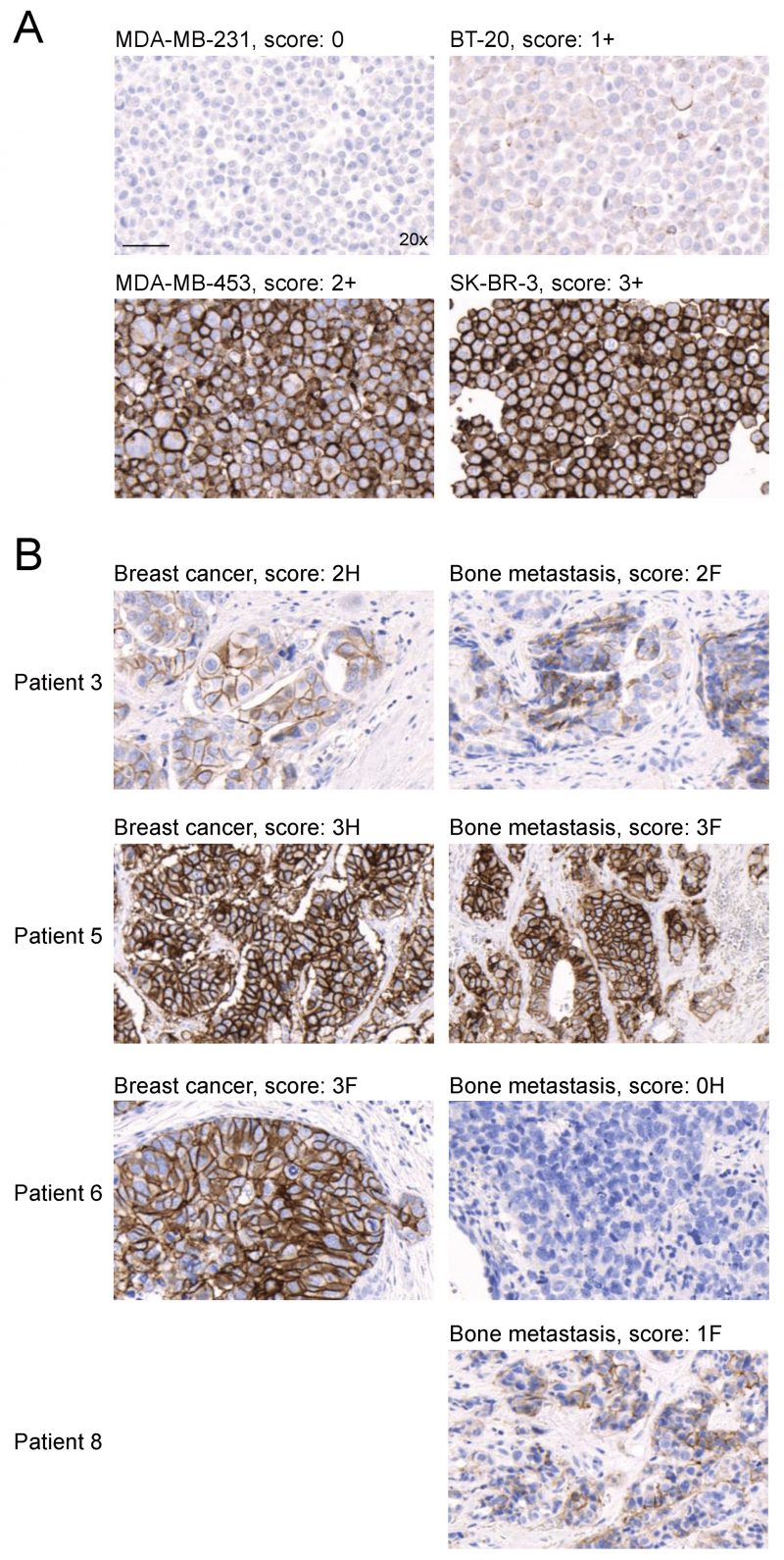
Figure 2. HER2 expression in matched primary breast cancer samples and bone metastasis samples from HER2-positive breast cancer patients. (A) HER2 expression in MDA-MB-231 (Score 0), BT-20 (Score 1+), MDA-MB-453 (Score 2+), and SK-BR-3 (Score 3+) breast cancer cells. HER2-positive breast cancer cells were stained as a reference. (B) Representative images of HER2 IHC analyses in breast cancer tissue and matched bone metastasis samples from four patients with HER2-positive primary breast cancer. The brown color indicates HER2 expression.
Precise Analysis with HSA KIT
The HSA KIT software offers a user-friendly interface with advanced annotation features for pixel-perfect precision. It promotes standardized and consistent procedures that enhance analysis quality.


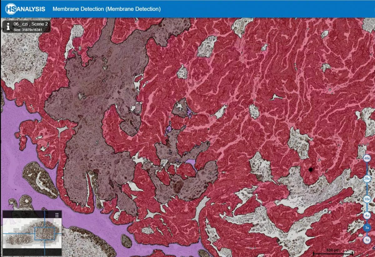
WSI zoomed out: Automatic detection of tumor areas (red), necrotic regions (brown), and stroma areas (purple).

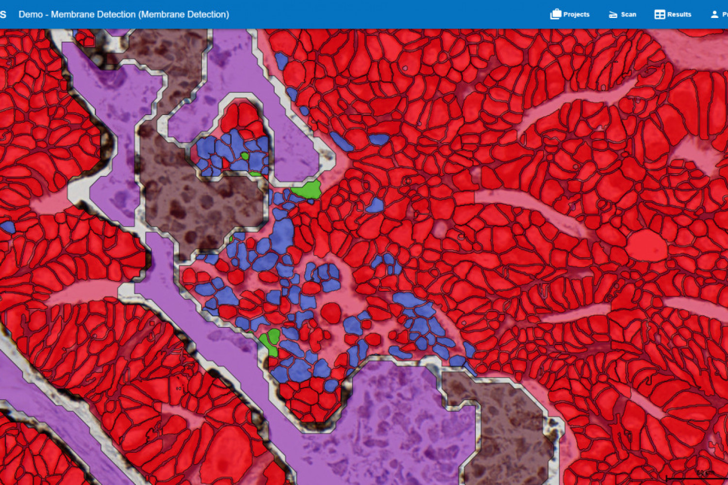
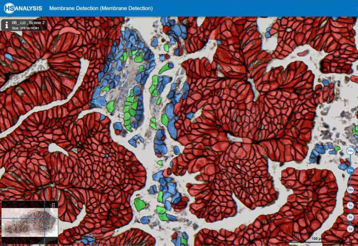
WSI zoomed in: Automatic detection of tumor areas (red), necrotic regions (brown), and stroma areas (purple) along with simultaneous detection and classification of tumor cells.


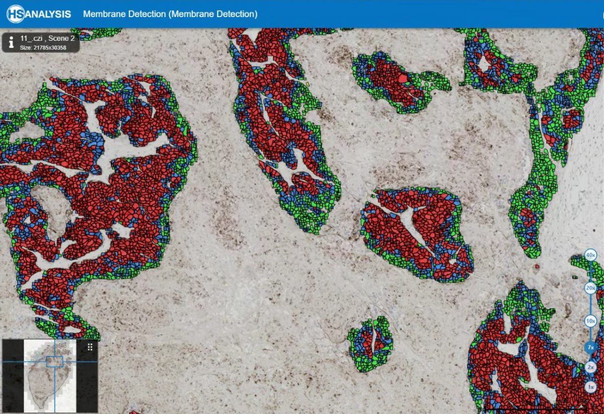
WSI zoomed in: Automatic classification of tumor cells into four classes.
In Figure 3, the different staining intensities from 0 to 3+ are shown. The H-Score can be based on a specific staining intensity or, more complexly, the sum of the individual H-Scores for each detected intensity. One method is to calculate the percentage of cells for each staining intensity and then assign an H-Score according to the formula provided in the link.
Detailed information about the result table and further calculations can be found here:
Area results
Total Area
The sum of all polygon areas.
$$\text{Total Area} = \sum_{i=1}^{n} \text{Area}_i$$
Percentage Area of Base ROI
The percentage of the total area of polygons relative to the base ROI.
$$\text{Percentage Area} = \left( \frac{\text{Total Area}}{\text{Base ROI Area}} \right) \times 100 \%$$
Minimum Area
The smallest polygon area.
$$\text{Minimum Area} = \min(\text{Area}_1, \text{Area}_2, \ldots, \text{Area}_n)$$
Maximum Area
The largest polygon area.
$$\text{Maximum Area} = \max(\text{Area}_1, \text{Area}_2, \ldots, \text{Area}_n)$$
Average Area
The mean area of all polygons.
$$\text{Average Area} = \frac{\sum_{i=1}^{n} \text{Area}_i}{n}$$
Median Area
The median area of all polygons.
$$\text{Median} =
\begin{cases}
\text{Area}_{\left(\frac{n+1}{2}\right)} & \text{if } n \text{ is odd} \\
\frac{\text{Area}_{\left(\frac{n}{2}\right)} + \text{Area}_{\left(\frac{n}{2} + 1\right)}}{2} & \text{if } n \text{ is even}
\end{cases}$$
Mode Area
The most frequently occurring area value.
$$\text{Mode Area} = \text{The value that appears most frequently in the dataset}$$
Standard Deviation (StdDev) Area
The measure of dispersion of polygon areas.
$$\text{StdDev} = \sqrt{\frac{1}{n} \sum_{i=1}^{n} (\text{Area}_i – \text{Average Area})^2}$$
Variance of Area
The square of the standard deviation.
$$\text{Variance} = \frac{1}{n} \sum_{i=1}^{n} (\text{Area}_i – \text{Average Area})^2$$
Mean Absolute Deviation of Area
The average of the absolute deviations from the mean.
$$\text{MAD} = \frac{1}{n} \sum_{i=1}^{n} |\text{Area}_i – \text{Average Area}|$$
Skewness
The measure of the asymmetry of the distribution of area values.
Kurtosis
The measure of the “tailedness” of the distribution of area values.
Object Size Quartiles (1st, 2nd, 3rd)
The quartile values of polygon areas.
Interquartile Range (1st – 3rd)
The range between the first and third quartile.
$$\text{IQR} = \text{Q3} – \text{Q1}$$
Decile Sizes (1st to 9th)
Values that divide the dataset into ten equal parts.
$$\text{D1} = \text{Area}_{\left(\frac{n+1}{10}\right)}$$
$$\text{D2} = \text{Area}_{\left(\frac{2(n+1)}{10}\right)}$$
$$\text{D3} = \text{Area}_{\left(\frac{3(n+1)}{10}\right)}$$
$$\text{D4} = \text{Area}_{\left(\frac{4(n+1)}{10}\right)}$$
$$\text{D5} = \text{Area}_{\left(\frac{5(n+1)}{10}\right)}$$
$$\text{D6} = \text{Area}_{\left(\frac{6(n+1)}{10}\right)}$$
$$\text{D7} = \text{Area}_{\left(\frac{7(n+1)}{10}\right)}$$
$$\text{D8} = \text{Area}_{\left(\frac{8(n+1)}{10}\right)}$$
$$\text{D9} = \text{Area}_{\left(\frac{9(n+1)}{10}\right)}$$
Confidence Intervals of Area
The range within which the true mean of the population lies with a certain confidence level.
$$\text{CI} = \text{Average Area} \pm (z \times \frac{\text{StdDev}}{\sqrt{n}})$$
Shape Factor
A measure of the compactness of the shape.
Area to Perimeter Ratio
The ratio of area to perimeter.
Eccentricity
The ratio of the distance between the foci of the ellipse and its major axis length.
$$\text{Eccentricity} = \sqrt{1 – \frac{b^2}{a^2}}$$
Other results
Object count
The number of polygons
Object density
The number of polygons per unit area.
$$\text{Object Density} = \frac{\text{Number of Polygons}}{\text{Total Area}}$$
Dispersion index
A measure of how polygons are dispersed over the area.
$$\text{Dispersion Index} = \frac{\text{Variance of Polygons per Unit Area}}{\text{Mean Polygons per Unit Area}}$$
Clustering analysis
A measure of how polygons are clustered together.
$$\text{Clustering Index} = \frac{\text{Variance of Polygons in Sub-regions}}{\text{Mean Polygons in Sub-regions}}$$
Maximum perimeter
The largest perimeter of the polygons.
$$\text{Maximum Perimeter} = \max(\text{Perimeter}_1, \text{Perimeter}_2, \ldots, \text{Perimeter}_n)$$
Average perimeter
The mean perimeter of all polygons.
$$\text{Average Perimeter} = \frac{\sum_{i=1}^{n} \text{Perimeter}_i}{n}$$
Median perimeter
The median perimeter of all polygons.
$$\text{Median Perimeter} =
\begin{cases}
\text{Perimeter}_{\left(\frac{n+1}{2}\right)} & \text{if } n \text{ is odd} \\
\frac{\text{Perimeter}_{\left(\frac{n}{2}\right)} + \text{Perimeter}_{\left(\frac{n}{2} + 1\right)}}{2} & \text{if } n \text{ is even}
\end{cases}$$stdev perimeter
The measure of dispersion of the perimeters of the polygons.
$$\text{StdDev Perimeter} = \sqrt{\frac{1}{n} \sum_{i=1}^{n} (\text{Perimeter}_i – \text{Average Perimeter})^2}$$
Variance of perimeter
The square of the standard deviation of the perimeters.
$$\text{Variance of Perimeter} = \frac{1}{n} \sum_{i=1}^{n} (\text{Perimeter}_i – \text{Average Perimeter})^2$$
Slide Scanner
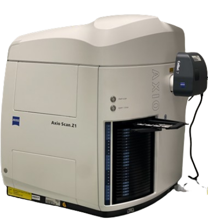
The HSA KIT can detect and analyze digitally generated microscopy images from slide scanners, such as the Axio Scan Z.1. It supports various image formats, including .tiff, .czi, and .jpg. The Axio Scan Z.1 allows for the scanning of tissue samples from various organs that have been prepared with different stains for specific cell membranes and biomarkers. This enables precise and detailed analysis of the captured image data.
Workflow with HSA KIT
Sample analysis and slide digitization have never been easier. The HSA KIT offers its customers an unparalleled experience for those looking to keep up with today’s “better” alternatives and achieve greater efficiency in their workflow. The HSA team goes above and beyond to satisfy its customers, from installation and integration of the software to unlimited support and upgrades.
Standardized process with subjective/objective analysis
Extraction of relevant features from raw data and creation of meaningful representations for training AI models
Module selection and configuration without excessive coding
Easy-to-learn software: Annotate, train, and automate
Quick and efficient analysis of multiple medical images, reducing time for diagnosis or treatment
Automatic report generation to increase productivity and assist doctors or radiologists in the evaluation process
We understand the importance of accurate and efficient slide analysis software. That’s why we offer a variety of features to help you achieve your goals.
Our software is compatible with both Linux and Windows operating systems and runs smoothly in Docker. With offline functionality, you can work on your slides without needing an internet connection, but if you want to expand to online use, that’s also possible.
We also offer professional integration into your network infrastructure, allowing you to seamlessly integrate our software into your existing systems.
Our software is designed to work with other programs as well, so you have all the tools you need at your disposal.
Even on weaker computers, our software delivers full performance, allowing you to analyze slides quickly and accurately.
And with the ability to generate reports in CSV and Excel formats, you have all the necessary data at your fingertips.
Finally, the user profile management ensures that the history and preferences of each user are saved for easy access.
AI-based analyses can be far more efficient, but they can only serve as a support tool for human expertise and never as a complete alternative. AI algorithms tend to produce false positives and false negatives and may struggle to adapt to data that deviates from the training datasets.
With our advanced technology and expert team, we are confident that we can deliver top-notch slide analysis services that meet the unique needs of each individual customer. Whether you’re looking for a one-time analysis or ongoing support, we have the tools and expertise to help you achieve your goals.


