Deep Learning (DL)
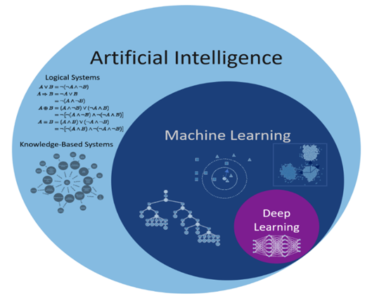
The connection between deep learning, machine learning, and AI. Artificial intelligence (AI) refers to techniques that enable computers to mimic human behavior. Using algorithms that have been trained on data, machine learning enables computers to classify or predict things. Deep learning is a type of machine learning that analyzes data and detects patterns using multi-layered neural networks, much like the way the human brain does. The structure of the human brain served as the inspiration for the neural network’s architecture.
Ground Truth Data (GTD)
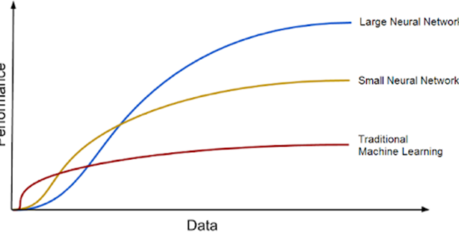
GTD refers to the real nature of the problem that a machine learning model is addressing and is required for the model to learn from labeled data. The more annotated the data, the better the algorithms will perform. Human evaluators or annotators must frequently produce ground truth labels in supervised learning algorithms, which may be costly and time consuming. The paper also compares GTD to ship engine fuel, with DL models serving as the engine and vast volumes of data serving as the fuel. With growing volumes of training data, DL models tend to improve, and the era of big data brings great prospects for future DL improvements.
Cost and Loss Function
The purpose of constructing a DL model is to reduce the difference between predicted and reality values. This is accomplished through the use of loss functions that are connected with each training example. The cost function is calculated by taking the average of the loss function values over all data samples. To decrease DL error, the cost function is optimized. We can attain the greatest outcomes in DL by improving the cost function.
Metrics
The matrices, which are useful for assessing the performance of machine learning models. When there are classification mistakes, confusion matrices are generated, and they have four possible values: True Positive, False Negative, False Positive, and True Negative. The confusion matrix may be used to determine classification metrics such as sensitivity, specificity, accuracy, negative predictive value, and precision.
Mean Average Precision (mAP)
The confusion matrix, Intersection over Union (IoU), recall, and precision are all part of the Mean Average Precision (mAP) calculation. It computes the weighted mean of precisions at each threshold, taking the increase in recall from the preceding threshold into consideration. The mAP is computed by calculating the AP for each class and then averaging the results over many classes. It is a helpful statistic for most detection applications since it gauges the trade-off between accuracy and recall.
Intersection over Union (IoU)
The standard commonly used to assess segmentation is Intersection over Union. This shows the overlap of the predicted bounding box coordinates with the ground truth box coordinates. A high IoU value indicates that the predicted bounding box coordinates are very similar to the ground truth box coordinates.
Creation of GTD
Selection of data set
In this work, the objective is to identify the most effective Deep Learning model for detecting colorectal cancer (CRC). Two distinct datasets are employed: one containing 1.6k annotations and another with 4.3k annotations. The primary aim is to investigate how the quantity of annotations influences the performance of our CRC detection model. To achieve this, separate training will be conducted using both datasets, allowing for a direct comparison of their respective performances. This analysis will enable us to ascertain whether having a larger number of annotations (4.3k) yields superior results in CRC detection compared to a smaller set of annotations (1.6k).
Deep learning models for CRC
After the creation of the GTD, to create the models, the steps to begin training for a deep learning model with the HSA KIT software. To begin, a model type must be chosen. This is referred to as instance segmentation or Segmentation. The structures on which the model should be trained must then be chosen. Then, in the “Augmentations” panel, you may indicate that alternative cell
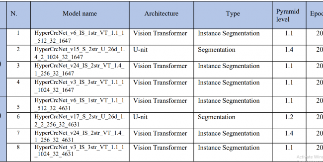
orientations are also detected. The model must then be given a name. After that, the model architecture, dataset settings, and hyperparameters for training the model are determined. Finally, the training can begin. Table below shows the different models that were trained.
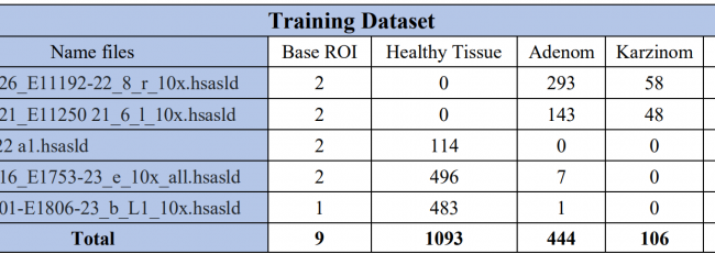
To generate ground truth data for training a deep learning model for colorectal cancer detection and classification, a multi-step process is followed. Initially, samples are acquired from individuals with colorectal cancer, typically in the form of tissue slides. These samples are then subjected to staining procedures such as Hematoxylin and Eosin (HE), Ki67, and CRC stains. The next crucial step involves the utilization of proprietary software, known as the HSA KIT. This software assists in automatically or manually defining the regions of interest (ROIs) within the samples. Within these ROIs, annotations are meticulously created using the HSA KIT tools, focusing on identifying colorectal cancer and categorizing it into three distinct structures: Healthy tissue, Adenoma, and Carcinoma. Furthermore, the final refinement of ground truth data involves manual annotation of the target areas within the selected ROIs, achieved by meticulously outlining the contours of the objects of interest. This comprehensive process ensures the availability of high-quality annotated data essential for training an accurate deep learning model for colorectal cancer analysis.
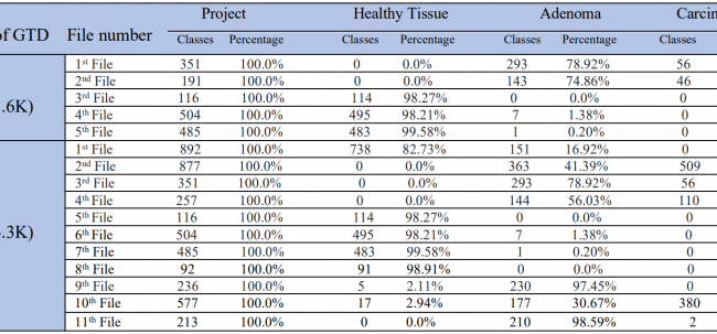
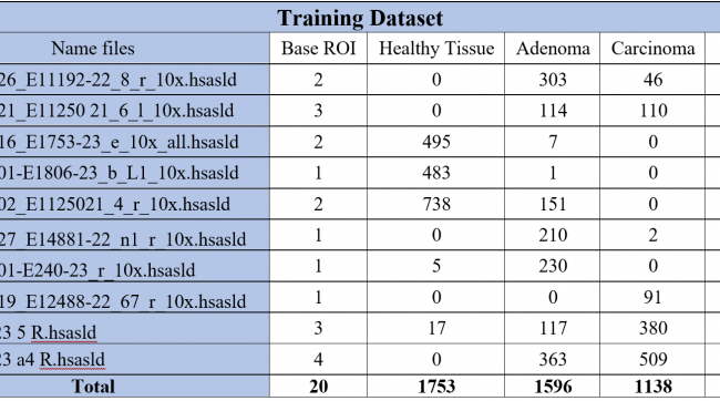
After creating the GTD, more GTDs were created to improve the model. The first time the model trained with 1647 GTD (1.6K). The second time the model trained with 4631 GTD (4.6K). The class distribution and their percentages in created data are given in the Table below.
Selection of data set
In this work, the objective is to identify the most effective Deep Learning model for detecting colorectal cancer (CRC). Two distinct datasets are employed: one containing 1.6k annotations and another with 4.3k annotations.
The primary aim is to investigate how the quantity of annotations influences the performance of our CRC detection model. To achieve this, separate training will be conducted using both datasets, allowing for a direct comparison of their respective performances.
This analysis will enable us to ascertain whether having a larger number of annotations (4.3k) yields superior results in CRC detection compared to a smaller set of annotations (1.6k).
Deep learning models for CRC
After the creation of the GTD, to create the models, the steps to begin training for a deep learning model with the HSA KIT software. To begin, a model type must be chosen. This is referred to as instance segmentation or Segmentation. The structures on which the model should be trained must then be chosen.
Then, in the “Augmentations” panel, you may indicate that alternative cell
orientations are also detected. The model must then be given a name. After that, the model architecture, dataset settings, and hyperparameters for training the model are determined.
Finally, the training can begin. Table below shows the different models that were trained.
Results
HyperCrcNet
The HSA KIT incorporates HyperCrcNet, a deep learning model tailored for colorectal cancer (CRC) imaging. HyperCrcNet has two versions:
- Type 1 based on the Vision Transformer (ViT) architecture, focuses on instance segmentation.
- Type 2 using the U-Net architecture, for segmentation.
Interpretation of trained model results
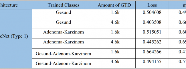
The settings presented in table below were selected to train the models. Loss and mAP were used to compare between models, where a lower loss and higher mAP are desirable characteristics for a better model. The loss and mAP of HyperCrcNet (Type 1) and HyperCrcNet (Type 2) models were compared with measured loss and IoU for the 1.6K and 4.6K GTD models.
Visual interpretation of the results
After the AI training is finished for any model, evaluating trained models are important for the user, we always have numerical evaluation. The trained model may have been tested numerically and it gives reasonable result. There will be always numbers as result and it is possible to have reasonable result by coincidence but actually could be wrong. That is the reason that before trusting the AI model, the result always has to be checked visually and not depend only on numbers. After creating trusted AI model, it can be used confidently, fully automated and under the control of AI. In this section the results will interpreted visually. And this section illustrates the visualization of the instance segmentation and segmentation of both of the (type 1 & 2) AI models of the CRC images.
Figure below displays a specific area without applying any model to it, including the “Gesund” structure.
is the same area with manual annotations specified by me. The result of HyperCrcNet (Type 1) both are the model trained with 1.6K and 4.6k GTD.

